All the Transformer Math You Need to Know | How To Scale Your Model

#TransformerModels #DeepLearning #NeuralNetworks #AI

All the Transformer Math You Need to Know

Part 4 of How To Scale Your Model (Part 3: Sharding | Part 5: Training)

Here we'll do a quick review of the Transformer architecture, specifically how to calculate FLOPs, bytes, and other quantities of interest.

Counting Dots

Let’s start with vectors $x$ , $y$ and matrices $A$ , $B$ of the following shapes:

a r r a y s h a p e x [P] y [P] A [N P] B [P M]

A dot product of $x \cdot y$ requires $P$ adds and multiplies, or $2 P$ floating-point operations total.
A matrix-vector product $A x$ does $N$ dot-products along the rows of $A$ , for $2 N P$ FLOPs.
A matrix-matrix product $A B$ does $M$ matrix-vector products for each column of $B$ , for $2 N P M$ FLOPs total.
In general, if we have two higher dimensional arrays $C$ and $D$ , where some dimensions are CONTRACTING and some are BATCHING. (e.g. $C [G H I J K L], D [G H M N K L]$ ) then the FLOPs cost of this contraction is two times the product of all of the $C$ and $D$ dimensions where the batch and contraction dimensions are only counted once, (e.g. $2 G H I J M N K L$ ). Note that a dimension is only batching if it occurs in both multiplicands. (Note also that the factor of 2 won’t apply if there are no contracting dimensions and this is just an elementwise product.)

O p e r a t i o n F L O P s D a t a x \cdot y 2 P 2 P A x 2 N P N P + P A B 2 N P M N P + P M [c 0, . . ., c N] \cdot [d 0, . . ., d N] 2 \prod c i \times \prod d j \notin B A T C H d j \notin C O N T R A C T d j \prod c i + \prod d j

Make note of the fact that for a matrix-matrix multiply, the compute scales cubically $O (N 3)$ while the data transfer only scales quadratically $O (N 2)$ - this means that as we scale up our matmul size, it becomes easier to hit the compute-saturated limit. This is extremely unusual, and explains in large part why we use architectures dominated by matrix multiplication - they’re amenable to being scaled!

Forward and reverse FLOPs

During training, we don’t particularly care about the result of a given matrix multiply; we really care about its derivative. That means we do significantly more FLOPs during backpropagation.

If we imagine B is just one matrix in a larger network and A are our input activations with C = A B, the derivative of the loss L with respect to B is given by the chain rule:

\partial L \partial B = \partial L \partial C \partial C \partial B = A T (\partial L \partial C)

which is an outer product and requires 2NPM FLOPs to compute (since it contracts over the N dimension). Likewise, the derivative of the loss with respect to A is

\partial L \partial A = \partial L \partial C \partial C \partial A = (\partial L \partial C) B T

is again 2NPM FLOPs since dL/dC is a (co-)vector of size $[N, M]$ . While this quantity isn’t the derivative wrt. a parameter, it’s used to compute derivatives for previous layers of the network (e.g. just as dL/dC is used to compute dL/dB above).

Adding these up, we see that during training, we have a total of 6NPM FLOPs, compared to 2NPM during inference: 2NPM in the forward pass, 4NPM in the backward pass. Since PM is the number of parameters in the matrix, this is the simplest form of the famous $6 * n u m p a r a m e t e r s * n u m t o k e n s$ approximation of Transformer FLOPs during training: each token requires $6 * n u m p a r a m e t e r s$ FLOPs. We’ll show a more correct derivation below.

Transformer Accounting

Transformers are the future. Well, they’re the present at least. Maybe a few years ago, they were one of many architectures. But today, it’s worth knowing pretty much every detail of the architecture. We won’t reintroduce the architecture but this blog and the original Transformer paper may be helpful references.

Here’s a basic diagram of the Transformer decoder architecture:

Figure: this diagram shows one layer of a standard Transformer and flows from top-to-bottom. We use a single-letter convention to describe the shapes and layouts of arrays in a Transformer, again showing contracting dimensions in red, and batched dimensions in blue. In a given operation, the input shape is given on top-left and the parameter shape is given on the top-right, with the resulting shape below, e.g. BTD is the input shape for the gating einsum and DF is the weight shape.

Note [gating einsum]: The diagram above uses a “ gating einsums ” where we split the up-projection matrix into two matrices (W_\text{In1} and W_\text{In2} above) whose outputs are elementwise multiplied as a kind of “gating function”. Not all LLMs use this, so you will sometimes see a single W_\text{In} matrix and a total MLP parameter count of 2DF instead of 3DF. Typically in this case, D and F will be scaled up to keep the parameter count the same as the 3 matrix case. With that said, some form of gating einsum is used by LLAMA, DeepSeek, and many other models.

Note 2 [MHA attention]: With self-attention, T and S are the same but for cross-attention they may be different. With vanilla Multi-Head Attention (MHA), N and K are the same while for Multi-Query Attention (MQA) K=1 and for Grouped MQA (GMQA) K merely has to divide N.

Global FLOPs and Params Calculation

For the below we’re going to compute per-layer FLOPs to avoid having to stick factors of L everywhere.

MLPs

The MLPs of a Transformer typically consist of 2 input matmuls that are element-wise combined and a single output matmul:

o p e r a t i o n t r a i n F L O P s p a r a m s A [B, T, D] \cdot W i n 1 [D, F] 6 B T D F D F A [B, T, D] \cdot W i n 2 [D, F] 6 B T D F D F σ (A i n 1) [B, T, F] * A i n 2 [B, T, F] O (B T F) A [B, T, F] \cdot W o u t [F, D] 6 B T D F D F \approx 18 B T D F 3 D F

Attention

For the generic grouped-query attention case with different Q and KV head numbers, let us assume equal head dimension H for Q,K,V projections, and estimate the cost of the QKVO matmuls:

o p e r a t i o n t r a i n F L O P s p a r a m s A [B, T, D] \cdot W Q [D, N, H] 6 B T D N H D N H A [B, T, D] \cdot W K [D, K, H] 6 B T D K H D K H A [B, T, D] \cdot W V [D, K, H] 6 B T D K H D K H A [B, T, N, H] \cdot W O [N, H, D] 6 B T D N H D N H 12 B T D (N + K) H 2 D (N + K) H

The dot-product attention operation is more subtle, effectively being a $T H \cdot H S$ matmul batched over the $B$ , $K$ dimensions, a softmax, and a $T S \cdot S H$ matmul again batched over the $B$ , $K$ dimensions. We highlight the batched dims in blue:

o p e r a t i o n t r a i n F L O P s Q [B, T, K, G, H] \cdot K [B, S, K, H] 6 B T S K G H = 6 B T S N H s o f t m a x S L [B, T, S, K, G] O (B T S K G) = O (B T S N) S [B, T, S, K, G] \cdot V [B, S, K, H] 6 B T S K G H = 6 B T S N H \approx 12 B T S N H = 12 B T 2 N H

Other Operations

There are several other operations happening in a Transformer. Layernorms are comparatively cheap and can be ignored for first-order cost estimates. There is also the final enormous (though not per-layer) unembedding matrix multiply.

o p e r a t i o n t r a i n F L O P s p a r a m s l a y e r n o r m D A [B, T, D] O (B T D) D A [B, T, D] \cdot W u n e m b e d [D, V] 6 B T D V D V

General rule of thumb for Transformer FLOPs

If we neglect the cost of dot-product attention for shorter-context training, then the total FLOPs across all layers is

(18 B T D F + 12 B T D (N + K) H) L = 6 * B T * (3 D F + 2 D (N + K) H) L = 6 * n u m t o k e n s * p a r a m e t e r c o u n t

Leading to a famous rule of thumb for estimating dense Transformer FLOP count, ignoring the attention FLOPs. (Unembedding is another simple matmul with 6BSDV FLOPs and DV params, and follows the same rule of thumb.)

Fractional cost of attention with context length

If we do account for dot-product attention above and assume $F = 4 D$ , $D = N H$ (as is typical) and $N = K$ :

a t t e n t i o n F L O P s m a t m u l F L O P s = 12 B T 2 N H 18 B T D F + 24 B T D N H = 12 B T 2 D 4 * 18 B T D 2 + 24 B T D 2 = 12 B T 2 D 96 B T D 2 = T 8 D

So the takeaway is that dot-product attention FLOPs only become dominant during training once T>8D. For D ~ 8k, this would be ~64K tokens. This makes some sense, since it means as the MLP size increases, the attention FLOPs become less critical. For large models, the quadratic cost of attention is not actually a huge obstacle to longer context training. However, for smaller models, even e.g. Gemma-27B, D=4608 which means attention becomes dominant around 32k sequence lengths. Flash Attention also helps alleviate the cost of long-context, which we discuss briefly in Appendix A.

Miscellaneous Math

Sparsity and Mixture-of-Experts

We’d be remiss not to briefly discuss Mixture of Experts (MoE) models, which replace the single dense MLP blocks in a standard Transformer with a set of independent MLPs that can be dynamically routed between. To a first approximation, an MoE is just a normal dense model with E MLP blocks per layer, instead of just one. Each token activates k of these experts, typically k=2. This increases the parameter count by O(E), while multiplying the total number of activated parameters per token by k, compared with the dense version.

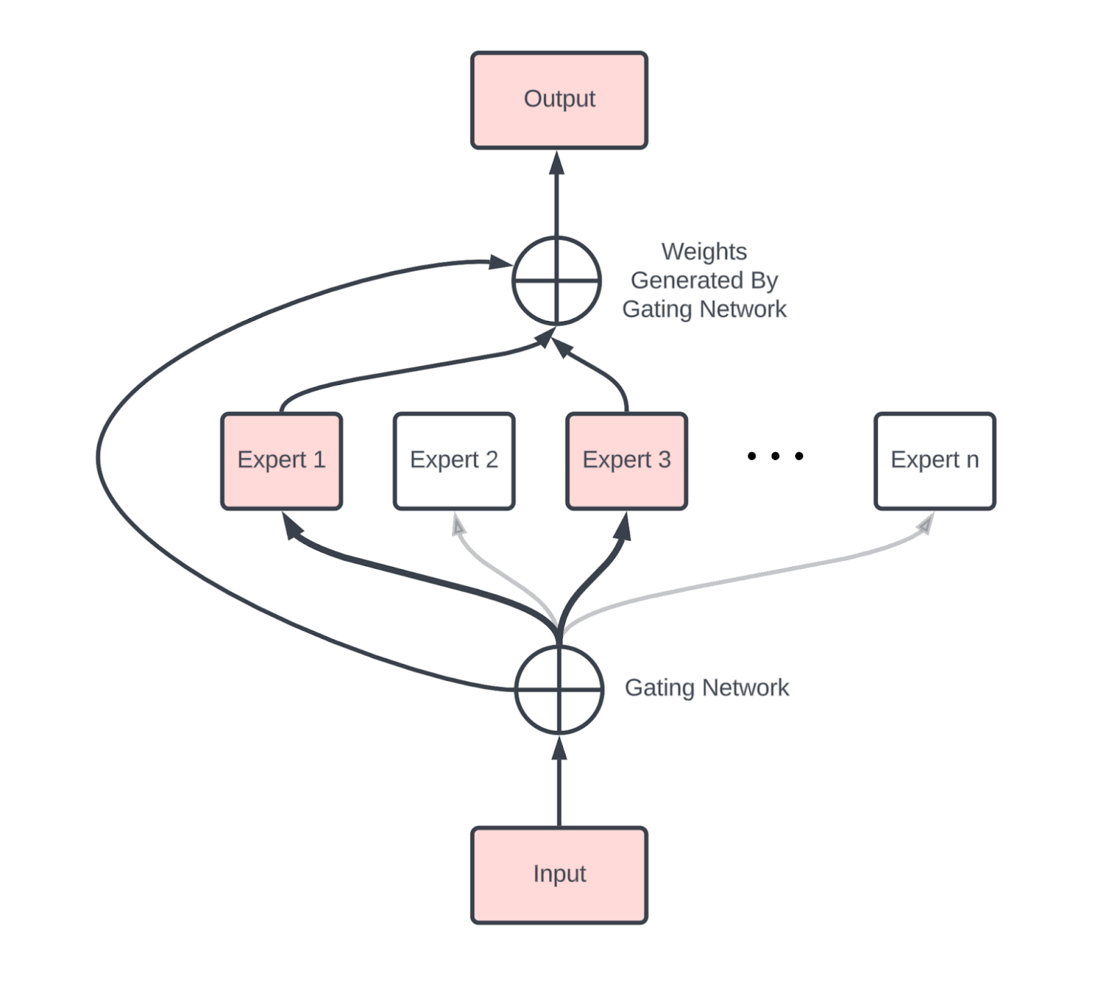
Figure: an example MoE layer with n experts. The gating expert routes each token to k of them, and the output of those MLPs get summed. Our parameter count is times the size of each expert, but only are used for each token. Source.

Compared to a dense model, an MoE introduces new comms, primarily two AllToAlls (one before and one after the MoE block) that route tokens to the correct expert and bring them back to their home device.Technically, this only happens if we are data or sequence sharded along the same axis as our experts. However as we saw in the previous section, the cost of each AllToAll is only 1/4 that of a comparable AllGather along a single axis (for a bidirectional ring).

Gradient checkpointing

Backpropagation as an algorithm trades memory for compute. Instead of a backward pass requiring $O (n l a y e r s 2)$ FLOPs, it requires $O (n l a y e r s)$ memory, saving all intermediate activations generated during the forward pass. While this is better than quadratic compute, it’s incredibly expensive memory-wise: a model with $B * T = 4 M$ (4M total tokens per batch), L=64, and D=8192 that avoids all unnecessary backward pass compute would have to save roughly $2 * 20 * B * T * D * L = 84 T B$ of activations in bfloat16. 20 comes from (roughly) counting every intermediate node in the Transformer diagram above, since e.g.

f (x) = e x p (g (x))

d f d x = e x p (g (x)) \cdot d g d x

so to avoid recomputing we need to save $g (x)$ and $e x p (g (x))$ from the forward pass. To avoid saving this much memory, we can choose to only save some fraction of the intermediate activations. Here are a few strategies we use.

Block remat: only save the input to each layer. This is the most aggressive method we use and only saves 1 checkpoint per layer, meaning we’d only save 4.2TB in the example above. This forces us to repeat essentially all forward pass FLOPs in the backward pass, meaning we increase our FLOPs from $6 N D$ to roughly $8 N D$ .
Big matmuls only: another simple policy is to only save the outputs of large matmuls. This lets us avoid recomputing any large matmuls during the backward pass, but still makes us recompute other activation functions and parts of attention. This reduces 20 per layer to closer to 7 per layer.

This by no means comprehensive. When using JAX, these are typically controlled by jax.remat / jax.checkpoint (you can read more here).

Key-Value (KV) caching

As we’ll see in Section 7, LLM inference has two key parts, prefill and generation.

Prefill processes a long prompt and saves its attention activations in a Key-Value Cache (KV Cache) for use in generation, specifically the key-value projections in the attention block.
Generation batches several of these KV caches together and samples tokens from each of them.

Each KV cache is then effectively an array of size [2, S, L, K, H] where the 2 accounts for the keys and values. This is quite large! The total size of the Key-Value cache in int8 is 2SLKH. For a moderately-sized model with 8k context length, 64 layers, and KH = NH = D = 8192, this is 2 \cdot 8192 \cdot 64 \cdot 8192 = 8\text{GiB}. You can see why we would want to use GMQA with K \ll N.

What Should You Take Away from this Section?

The overall parameters and FLOPs of a Transformer are fairly easy to calculate, and are summarized here, assuming MHA (with batch size B, vocab size V, a sequence of length T, D=d _model, and F=d _ff):

Component	Params per layer	Training FLOPs per layer
MLP	3DF	18BTDF
Attention	4DNH	24BTDNH + 12BT ² NH
Other	D	BTD
Vocab	DV (total, not per-layer)	12BTDV

The parameter count of the MLP block dominates the total parameter count and the MLP block also dominates the FLOPs budget as long as the sequence length T < 8D.
The total FLOPs budget during training is well approximated by $6 \cdot n u m_{p} a r a m s \cdot n u m_{t} o k e n s$ for reasonable context lengths.
During inference, our KV caches are roughly $2 \cdot S \cdot L \cdot N \cdot H$ per cache, although architectural modifications can often reduce this.

A Few Problems to Work

Question 1: How many parameters does a model with D=4096, F=4 \cdot D, V=32,000, and L=64 have? What fraction of these are attention parameters? How large are our KV caches per token? You can assume N\cdot H=D and multi-head attention with int8 KVs.

Click here for the answer.

The total parameters is roughly $L \cdot (3 D F + 4 D N H + D) + 2 D V$ . For the given numbers, this is $64 \cdot (3 \cdot 4 e 3 \cdot 16 e 3 + 4 \cdot 4 e 3 \cdot 4 e 3 + 4 e 3) + 2 \cdot 4 e 3 \cdot 32 e 3 = 16 e 9$ , or 16B parameters.
The ratio of attention parameters to total parameters in general is $4 D N H / (4 D N H + 3 D F) = 4 D 2 / (4 D 2 + 12 D 2) = 1 / 4$ . This gives us roughly 1/4 of parameters are used in attention.
Per token, our KV caches are $2 \cdot L \cdot N \cdot H = 2 \cdot 64 \cdot 4096$ in int8, which is 512kB / token.

Question 2: How many total FLOPs are required to perform A[B _X, D _Y] * _D W[D _Y, F] on {‘X': 4, ‘Y': 8, ‘Z': 4}. How many FLOPs are performed by each TPU?

Click here for the answer.

The total “theoretical” FLOPs of the operation is $2 \cdot B \cdot D \cdot F$ . However, because the computation isn’t sharded across the Z dimension, we’re actually doing Z extra FLOPs, meaning $2 \cdot B \cdot D \cdot F \cdot Z$ total FLOPs. Since the computation is sharded across the other dimensions, the total per-device is roughly $2 \cdot B \cdot D \cdot F / (X \cdot Y)$ .

Question 3: How many FLOPs are involved in performing A[I,J,K,L] * B[I,J,M,N,O] \rightarrow C[K,L,M,N,O]?

Click here for the answer.

Following the rule above, we have I and J as contracting dimensions and K, L, M, N, and O as non-contracting dimensions. We have no “batching dimensions”, so this is just $2 \cdot I \cdot J \cdot K \cdot L \cdot M \cdot N \cdot O$ , the sum of all the axes. If we had a shared axis, it would only be counted once.

Question 4: What is the arithmetic intensity of self-attention (ignoring the Q/K/V/O projections)? Give the answer as a function of the Q and KV lengths T and S. At what context length is attention FLOPs-bound? Given the HBM bandwidth of our TPUs, plot the effective relative cost of attention to the FFW block as the context length grows.

Click here for the answer.

Self-attention requires loading the $Q$ , $K$ , and $V$ activations, then computing $s o f t m a x (Q \cdot K) \cdot V$ , then writing the result back to HBM. This will be done with Flash Attention so there are some caveats to this math, but basically in bf16 self-attention performs

Q [B, T, N, H] \to r e s h a p e Q [B, T, K, G, H] \cdot K [B, S, K, H] \to O [B, T, S, K, G]

U = s o f t m a x S (O [B, T, S, K, G])

U [B, T, S, K, G] \cdot V [B, S, K, H] \to X [B, T, K, G, H]

So our total bytes is $2 * s i z e o f (Q) + 2 * s i z e o f (K o r V) = 4 B T N H + 4 B S K H = 4 B H K * (T G + S)$ , total FLOPs is $4 B T S N H + O (B T S N)$ and the arithmetic intensity is $4 B T S K G H / (4 B H K * (T G + S))$ .

So basically, during prefill we have $S = T$ so we have an arithmetic intensity of $4 B T 2 K G H / 4 B H K T \cdot (G + 1) = T G / (G + 1) = O (T)$ . During generation, $T = 1$ so we have $4 B S K G H / (4 B H K \cdot (G + S)) = S G / (G + S) \to G$ assuming $S$ is very large. Depending on how you interpret the question, during prefill or training self-attention is compute bound at S=240 assuming no sequence sharding. During generation, we are never compute bound because $G$ is small. Nonetheless, however, you can see that increasing $G$ leads to us being closer to compute bound.

Question 5: At what sequence length are self-attention FLOPs equal to the QKVO projection FLOPs?

Click here for the answer.

This is purely a question of when $24 B T D N H == 12 B T 2 N H$ . Simplifying we get $2 D = T$ , so e.g. for $D = 4096$ , this is $8192$ . This tells us that for most reasonable context lengths, matmul FLOPs are greater.

Question 6: Say we only save the output of each of the 7 main matmuls in a Transformer layer during our forward pass (Q, K, V, O + the three FFW matrices). How many extra FLOPs do we need to “rematerialize” during the backwards pass?

Question 7: DeepSeek v3 says it was trained for 2.79M H800 hours on 14.8T tokens (source). Given that it has 37B activated parameters, roughly what hardware utilization did they achieve? Hint: note that they used FP8 FLOPs without structured sparsity.

Click here for the answer.

From the spec sheet here, we find 3,026 TFLOPs/s of FP8 performance with sparsity, or typically half this (1.513e15 FLOPs/s) without sparsity. 2.79M H800 hours means 2.79e6 * 1.513e15 * 60 * 60 = 1.52e25 total FLOPs. Given the activated parameter count of 37B, this training run should have used about 6 * 37e9 * 14.8e12 = 3.3e24 FLOPs. That means the FLOPs utilization is about 3.3e24 / 1.52e25 = 21.7%.

Question 8: Mixture of Experts (MoE) models have E copies of a standard dense MLP block, and each token activates k of these experts. What batch size in tokens is required to be compute-bound for an MoE with weights in int8 on TPU v5e? For DeepSeek, which has 256 (routed) experts and k=8, what is this number?

Click here for the answer.

Because we have E copies of each expert, in int8, we need to load E \cdot D \cdot F bytes. Because each token activates k experts, we have 2\cdot k \cdot B \cdot D \cdot F FLOPs. To be compute-bound with bfloat16 FLOPs, we need an arithmetic intensity over 240 which happens when (2\cdot k \cdot BDF) / EDF > 240 or k \cdot B / E > 120.

Therefore, we need B > 120 \cdot E / k to be compute bound. For DeepSeek, this gives us B > 120 \cdot 256 / 8 = 3840. This is a remarkably large batch size at generation time.

The traditional objection to scaling Transformers to very long context is that the attention FLOPs and memory usage scale quadratically with context length. While it’s true that the attention QK product has shape [B, S, T, N] where B is the batch size, S and T are the Q and K sequence dims, and N is the number of heads, this claim comes with some serious caveats:

As we noted in Section 4, even though this is quadratic, the attention FLOPs only dominated when $S > 8 \cdot D$ , and especially during training the memory of a single attention matrix is small compared to all of the weights and activation checkpoints living in memory, especially when sharded.
We don’t need to materialize the full attention matrix in order to compute attention! We can compute local sums and maxes and avoid ever materializing more than a small chunk of the array. While the total FLOPs is still quadratic, we drastically reduce memory pressure.

This second observation was first made by Rabe et al. 2021 and later in the Flash Attention paper (Dao et al. 2022). The basic idea is to compute the attention in chunks of K/V, where we compute the local softmax and some auxiliary statistics, then pass them onto the next chunk which combines them with its local chunk. Specifically, we compute

M: The running max of $q \cdot k$ over the sequence dimension
O: The running full attention softmax over the sequence dimension
L: The running denominator $\sum i (q \cdot k i - r u n n i n g m a x)$

With these, we can compute the new max, the new running sum, and the new output with only a constant amount of memory. To give a sketchy description of how this works, attention is roughly this operation:

A t t n (Q, K, V) = \sum i e x p (Q \cdot K i - m a x j Q \cdot K j) V i \sum l e x p (Q \cdot K l - m a x j Q \cdot K j)

The max is subtracted for numerical stability and can be added without affecting the outcome since $\sum i e x p (a i + b) = e x p (b) \sum e x p (a)$ . Looking just at the denominator above, if we imagine having two contiguous chunks of key vectors, $K 1$ and $K 2$ and we compute the local softmax sums $L 1$ and $L 2$ for each

L 1 = \sum i e x p (Q \cdot K i 1 - m a x j Q \cdot K j 1)

L 2 = \sum i e x p (Q \cdot K i 2 - m a x j Q \cdot K j 1)

Then we can combine these into the full softmax sum for these two chunks together by using

L c o m b i n e d = e x p (M 1 - m a x (M 1, M 2)) \cdot L 1 + e x p (M 2 - m a x (M 1, M 2)) \cdot L 2

where

M 1 = m a x j Q \cdot K j 1 a n d M 2 = m a x j Q \cdot K j 2

This can be done for the full softmax as well, giving us a way of accumulating arbitrarily large softmax sums. Here’s the full algorithm from the Flash Attention paper.

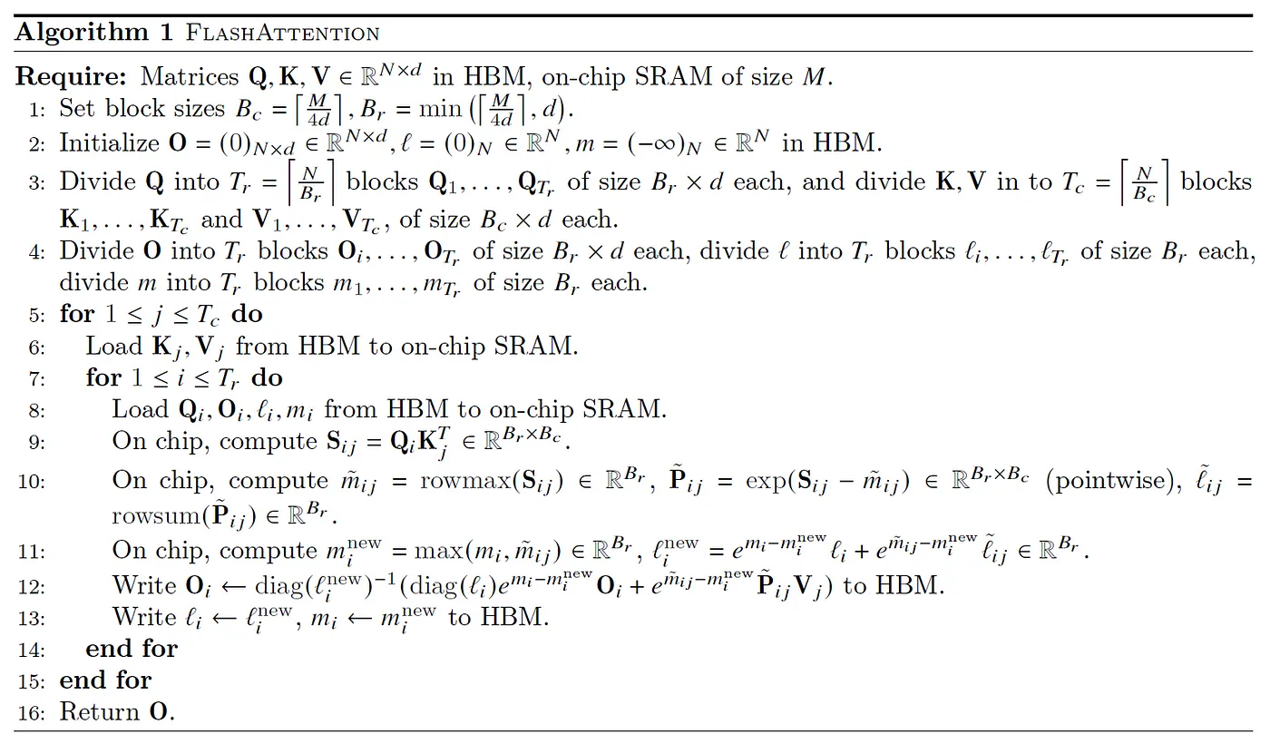
From a hardware standpoint, this lets us fit our chunk of Q into VMEM (what the algorithm above calls on-chip SRAM) so we only have to load the KV chunks on each iteration, reducing the arithmetic intensity. We can also keep the running statistics in VMEM.

One last subtle point worth emphasizing is an attention softmax property that’s used to make the Flash VJP (reverse mode derivative) calculation practical for training. If we define an intermediate softmax array as:

S i j = e τ q i \cdot k j \sum k e τ q i \cdot k j

In attention, we obtain dS from reverse-mode dO and V arrays:

d S i j = d O i d \cdot d V j d = \sum d d O i d V j d

During the backpropagation of this gradient to Q and K

d (q i \cdot k j) = (d S i j - S i j \cdot j d S i j) S i j

We exploit an identity that allows us to exchange a contraction along the large key length dimension with a local contraction along the feature depth dimension.

S i j \cdot j d S i j = \sum j e τ q i \cdot k j \sum k e τ q i \cdot k k \sum d d O i d V j d = \sum d d O i d \sum j e τ q i \cdot k j \sum k e τ q i \cdot k k V j d = \sum d d O i d O i d = d O i d \cdot d O i d

This replacement is crucial for being able to implement a sequence-block local calculation for the VJP, and enables further clever sharding schemes like ring attention.

Footnotes

Technically, this only happens if we are data or sequence sharded along the same axis as our experts.

All the Transformer Math You Need to Know | How To Scale Your Model